Building an Interactive Data Exploration App with R Shiny

Introduction

In this tutorial, we will walk through the creation of an interactive data exploration application using R Shiny. This app allows users to filter data, view various charts, and download them for further analysis.

Prerequisites

  • Basic understanding of R programming
  • R and RStudio installed
  • Shiny, ggplot2, and DT packages installed

App Overview

Our R Shiny app includes:

  • A filterable table
  • Interactive charts including bar plots, scatter plots, and line plots
  • Data download functionality

Getting Started

First, ensure you have the required libraries:

library(shiny)
library(DT)
library(ggplot2)

Data Preparation

Load and preprocess your data. In our case, we are reading from a CSV file and creating bins for age and income:

dataset = read.csv("dataset.csv")
# Create bins for age and income
dataset$AGE_Bin = cut(dataset$AGE,5,include.lowest = TRUE)
dataset$INCOME_Bin = cut(dataset$INCOME,5,include.lowest = TRUE,dig.lab = 6)

The code contains the UI and Server in two parts. I will layout the complete code of each part here, and later in the article, I will delve into the very intuitive UI design in Shiny.

Building the UI

The user interface (UI) is designed with fluidPage for a responsive layout.

ui <-   fluidPage(
    
    h1("Rshiny Homework"),
    h2("Demographic Exploartion"),
    h3("Filterable Table"),
    DT::dataTableOutput("table"),
    br(),
    h3("Charts"),
    selectInput(
        "option",
        "Demography",
        c("AGE_Bin","INCOME_Bin","GENDER"),
        selected = NULL,
        multiple = FALSE,
        selectize = TRUE,
        width = NULL,
        size = NULL
    ),
    
    actionButton("gobutton", "View Chart", class = "btn-success"),
    plotOutput("disPlot"),
    downloadButton(outputId = "disPlot_download", label = "Download Chart",class = "btn-success"),
    
    br(),
    hr(),
    br(),
    h3("Relationship Between Variables"),
    
    tabsetPanel(
        tabPanel("Scatter", 
                 plotOutput("Scatter", brush="selected_range"),
                 br(),
                 downloadButton(outputId = "scatter_download", label = "Download Chart",class = "btn-success"),
                 br(),
                 br(),
                 DT::dataTableOutput("brushed_table")
        ),
        tabPanel("Distribution", 
                 plotOutput("displot2"),
                 downloadButton(outputId = "displot2_download", label = "Download Chart",class = "btn-success"),
                 br(),
                 plotOutput("displot3"),
                 downloadButton(outputId = "displot3_download", label = "Download Chart",class = "btn-success")
                 
        )
    ),
    
    br(),
    hr(),
    br(),
    h3("Line Plot"),
    plotOutput("lineplot"),
    downloadButton(outputId = "lineplot_download", label = "Download Chart",class = "btn-success"),
    br(),
    plotOutput("lineplot2"),
    downloadButton(outputId = "lineplot2_download", label = "Download Chart",class = "btn-success")
)

Server Logic

The server function contains the logic for rendering plots and tables based on user input. As you may find, all backend data handling and visual design goes in here.

server <- function(input,output, session) {
    
    library(ggplot2)
    library(shiny)
    library(DT)
    # library(stringr)
    
    #setwd("C:/Users/kli4/Downloads/Shiny_HW")
    
    dataset = read.csv("dataset.csv")
    dataset$AGE_Bin = cut(dataset$AGE,5,include.lowest = TRUE)
    dataset$INCOME_Bin = cut(dataset$INCOME,5,include.lowest = TRUE,dig.lab = 6)
    # dataset$INCOME_Bin <- lapply(strsplit(gsub("]|[[(]", "", levels(dataset$INCOME_Bin)), ","),
    #           prettyNum, big.mark=".", decimal.mark=",", input.d.mark=".", preserve.width="individual")
    
    
    plot_var <- eventReactive(input$gobutton,{
        
        selection <- input$option
        
        data_agg <-aggregate(x=dataset$Customer, by=list(SELECTION=dataset[,c(selection)],TREATMENT = dataset[,"TREATMENT"]),length)
        names(data_agg) = c("SELECTION","TREATMENT", "Customer")
        
        return(data_agg)
        
    })
    
    
    output$disPlot <- renderPlot({
        displot = ggplot(plot_var(), aes(x=SELECTION,y=Customer,fill=TREATMENT)) + geom_bar(position="stack",stat="identity")
        
        output$disPlot_download <- downloadHandler(
            filename = function() { paste(input$option, '.jpg', sep='') },
            content = function(file){
                ggsave(file,plot=displot)
            })
        displot
    })
    

    output$table <- DT::renderDataTable(datatable(dataset))
 
    scatter_plot <- ggplot(dataset, aes(x=AGE,y=INCOME)) + geom_point()
    
    scatter_plot = scatter_plot + facet_grid(GENDER ~ TREATMENT)
    
    output$Scatter <- renderPlot({
        scatter_plot
    })
    
    scatter_brushed <- reactive({
        
        my_brush <- input$selected_range
        sel_range <- brushedPoints(dataset, my_brush)
        return(sel_range)
        
    })
    output$brushed_table <- DT::renderDataTable(DT::datatable(scatter_brushed()))


    displot2 <- ggplot(dataset, aes(online.Activity.A)) + geom_histogram(aes(fill=AGE_Bin), bins = 5)
    
    displot2 = displot2 + facet_grid(GENDER ~ TREATMENT)
    
    displot3 <- ggplot(dataset, aes(online.ACTIVITY.B)) + geom_histogram(aes(fill=AGE_Bin), bins = 5)
    
    displot3 = displot3 + facet_grid(GENDER ~ TREATMENT)
    
    output$displot2 <- renderPlot({
        displot2
    })
    
    output$displot3 <- renderPlot({
        displot3
    })
    # 
    # scatter_brushed2 <- reactive({
    #   
    #   my_brush <- input$selected_range2
    #   sel_range <- brushedPoints(dataset, my_brush)
    #   return(sel_range)
    #   
    # })
    # output$brushed_table2 <- DT::renderDataTable(DT::datatable(scatter_brushed2()))
    
    data_agg2 <-aggregate(list(Activity_A=dataset$online.Activity.A), by=list(DAY=dataset$DAY,TREATMENT=dataset$TREATMENT,GENDER=dataset$GENDER),mean)
    
    lineplot <- ggplot(data_agg2, aes(x=DAY, y=Activity_A, group=c(TREATMENT))) + geom_line(aes(color=TREATMENT)) + geom_point()
    lineplot = lineplot + facet_grid(GENDER ~ TREATMENT)
    
    output$lineplot <- renderPlot({
        lineplot
    })
    
    data_agg2 <-aggregate(list(Activity_B=dataset$online.ACTIVITY.B), by=list(DAY=dataset$DAY,TREATMENT=dataset$TREATMENT, GENDER=dataset$GENDER),mean)
    
    lineplot2 <- ggplot(data_agg2, aes(x=DAY, y=Activity_B, group=c(TREATMENT))) + geom_line(aes(color=TREATMENT)) + geom_point()
    lineplot2 = lineplot2 + facet_grid(GENDER ~ TREATMENT)
    
    output$lineplot2 <- renderPlot({
        lineplot2
    })
    
    #Downloads
    
    output$lineplot2_download <- downloadHandler(
        filename = "Activity_B Line.jpg",
        content = function(file){
            ggsave(file,plot=lineplot2)
        })
    
    output$lineplot_download <- downloadHandler(
        filename = "Activity_A Line.jpg",
        content = function(file){
            ggsave(file,plot=lineplot)
        })
    
    output$displot2_download <- downloadHandler(
        filename = "ActivityA_Dist.jpg",
        content = function(file){
            ggsave(file,plot=displot2)
        })
    output$displot3_download <- downloadHandler(
        filename = "ActivityB_Dist.jpg",
        content = function(file){
            ggsave(file,plot=displot3)
        })
    
    output$scatter_download <- downloadHandler(
        filename = "Age_Income.jpg",
        content = function(file){
            ggsave(file,plot=scatter_plot)
        })
    

}

UI Design in R Shiny

UI design in R Shiny is easy and intuitive. It’s an HTML element as a function concept. Let’s dive into how UI is designed in our R Shiny app, using the provided code as an example.

Basic Structure

R Shiny UI is structured using functions defining the layout and its elements. The fluidPage() function is often used for its responsive layout capabilities, meaning the app’s interface adjusts nicely to different screen sizes.

ui <- fluidPage(
    # UI components are nested here
)

Organizing Content with Headers and Separators

Headers (h1, h2, h3, etc.) and separators (hr()) are used to organize content and improve readability. In our app, headers indicate different sections:

h1("Rshiny Homework"),
h2("Demographic Exploration"),
h3("Filterable Table"),

Data Display

The DT::dataTableOutput() function is used to render data tables in the UI. This function takes an output ID as an argument, linking it to the server logic that provides the data:

DT::dataTableOutput("table"),

Interactive Inputs

Interactive inputs, such as selectInput, allowing users to interact with the app and control what data or plot is displayed. In our app, selectInput is used for choosing demographic aspects to display in a chart:

selectInput(
    "option",
    "Demography",
    c("AGE_Bin", "INCOME_Bin", "GENDER"),
    selected = NULL,
    multiple = FALSE,
    selectize = TRUE,
    width = NULL,
    size = NULL
),

Action Buttons

Action buttons, created with actionButton(), trigger reactive events in the server. Our app uses an action button to generate plots based on user selection:

actionButton("gobutton", "View Chart", class = "btn-success"),

Displaying Plots

To display plots, plotOutput() is used. This function references an output ID from the server side where the plot is rendered:

plotOutput("disPlot"),

Interactive Plots

I use ggplot2 for creating interactive plots. For example, a scatter plot is generated based on user-selected variables:

scatter_plot <- ggplot(dataset, aes(x=AGE,y=INCOME)) + geom_point()

Tabbed Panels

Tabbed panels, created with tabsetPanel(), help in organizing content into separate views within the same space. Each tabPanel holds different content:

tabsetPanel(
    tabPanel("Scatter", ...),
    tabPanel("Distribution", ...)
),

Download Handlers

We provide functionality for users to download plots as JPEG files:

output$scatter_download <- downloadHandler(
    filename = "Age_Income.jpg",
    content = function(file){
        ggsave(file,plot=scatter_plot)
    })

downloadButton(outputId = "scatter_download", label = "Download Chart", class = "btn-success"),

Running the App

Finally, to run the app, use:

shinyApp(ui = ui, server = server)

Run Regression in Python with Statsmodel Package

Run Regression
In [9]:
from statsmodels import api as sm
from my_libs import *

Regress the SPY and VIX index

  • Need to translate the result into np.array
  • Need to change type to float
In [51]:
spy = get_price_data(["SPY"],method='day',back_day=20).dropna().Return.values.astype(float)
spy_ = spy*30
All price data of Close is actually Adj Close
Connection Successful
Finished SPY

Constructed a model of vix = intercept + b0 * spy + b1 * spy * 30

In [52]:
ip = pd.DataFrame({"spy":spy,"spy_":spy_})
dp = get_price_data(["^VIX"],method='day',back_day=20).dropna().Return.values.astype(float)
All price data of Close is actually Adj Close
Connection Successful
no data for ^VIX
'NoneType' object has no attribute 'index'
switching to realtimeday method
Finished ^VIX
In [53]:
ip = sm.add_constant(ip)
/home/ken/.local/lib/python2.7/site-packages/numpy/core/fromnumeric.py:2389: FutureWarning: Method .ptp is deprecated and will be removed in a future version. Use numpy.ptp instead.
  return ptp(axis=axis, out=out, **kwargs)
In [54]:
sm.OLS(dp,ip).fit().summary()
/home/ken/.local/lib/python2.7/site-packages/scipy/stats/stats.py:1416: UserWarning: kurtosistest only valid for n>=20 ... continuing anyway, n=13
  "anyway, n=%i" % int(n))
Out[54]:
OLS Regression Results
Dep. Variable: y R-squared: 0.737
Model: OLS Adj. R-squared: 0.713
Method: Least Squares F-statistic: 30.80
Date: Sun, 04 Aug 2019 Prob (F-statistic): 0.000173
Time: 19:40:53 Log-Likelihood: 25.241
No. Observations: 13 AIC: -46.48
Df Residuals: 11 BIC: -45.35
Df Model: 1
Covariance Type: nonrobust
coef std err t P>|t| [0.025 0.975]
const 0.0033 0.011 0.305 0.766 -0.021 0.027
spy -0.0109 0.002 -5.550 0.000 -0.015 -0.007
spy_ -0.3256 0.059 -5.550 0.000 -0.455 -0.196
Omnibus: 9.222 Durbin-Watson: 1.071
Prob(Omnibus): 0.010 Jarque-Bera (JB): 4.912
Skew: -1.262 Prob(JB): 0.0858
Kurtosis: 4.641 Cond. No. 5.85e+17


Warnings:
[1] Standard Errors assume that the covariance matrix of the errors is correctly specified.
[2] The smallest eigenvalue is 3.82e-35. This might indicate that there are
strong multicollinearity problems or that the design matrix is singular.

Set up AWS Lightsail for Multiple WordPress Sites

This is a documentation of creating an AWS account, setting up a Lightsail (one of the functions offered by AWS) resource, and installing multiple WordPress websites. I will be covering the following topics:

  • Creating an AWS account and navigating through the dashboard of AWS
  • Setting up Lightsail LAMP Linux instance and Statics IP
  • Using SSH to connect to the terminal
  • Setting server configuration for WordPress
  • Installing WordPress
  • Create SSL Certification using Let’s Encrypt

Creating AWS Account

First of all, you need an AWS account to get started Simply visit aws.amazon.com and click “Sign in to the Console”, then register a new account. To get the account active and be able to set up Lightsail, you fill in credit information for the account. It usually takes them overnight to verify the account. If longer than that, I suggest you contact them. For corporate account, they may need to call in and verify company information.

Once the account is verified, you can set up Lightsail as followed.

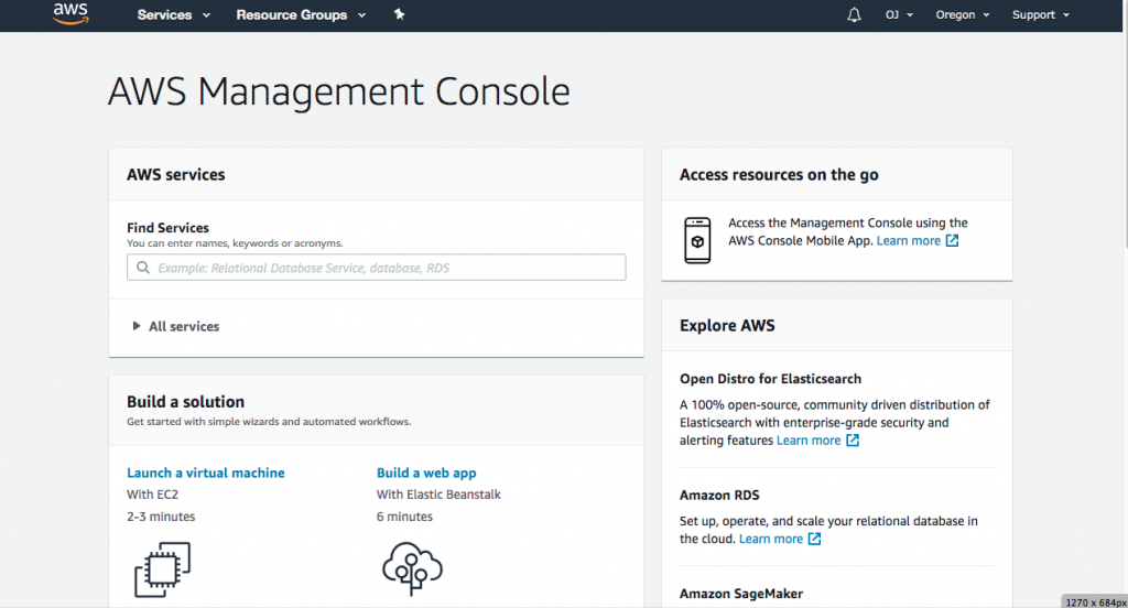
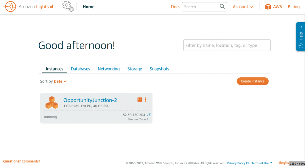
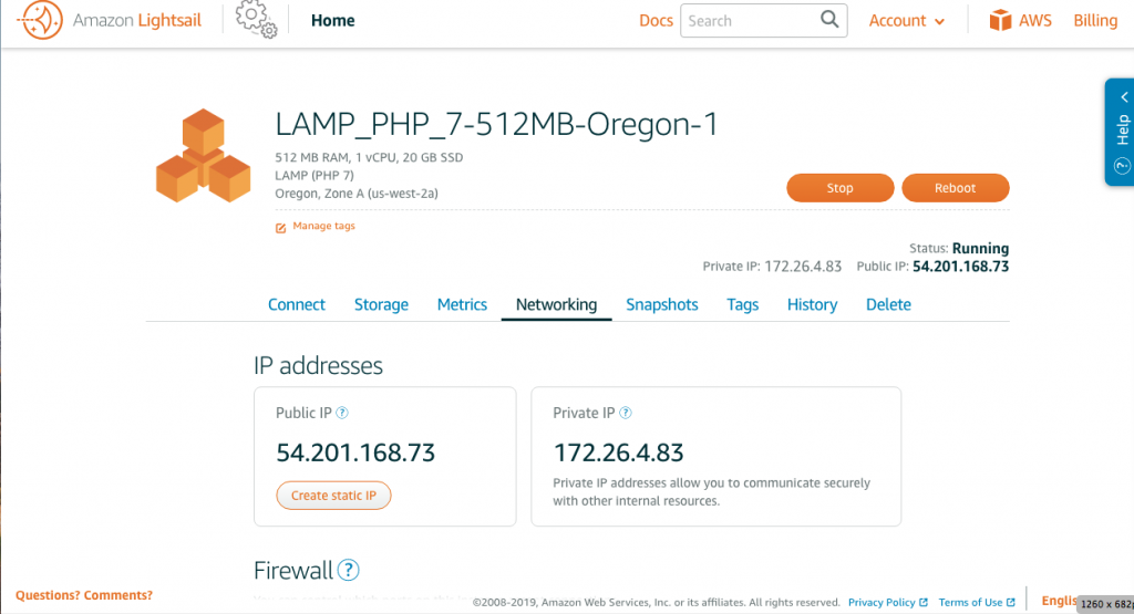
Click Services on the top bar and select Lightsail (usually on the first column). When you land on Lightsail page you will see something like this.

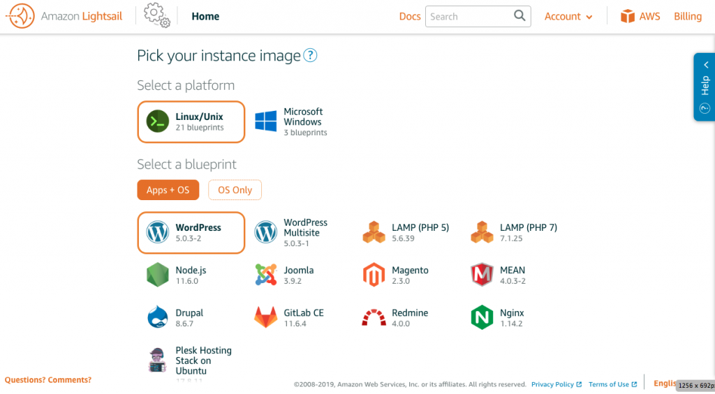
When you create an instance, here’s what you will see.

To create a stable multisite instance without purchasing expensive plugin (especially the All-in-one backup) to support WordPress Multisite, in this documentation, we will create a LAMP (PHP 7) to build from scratch. After choosing the image, you will be asked to choose a plan. After it’s done, you will see an instance showed up on your Lightsail dashboard.

The first thing to do after creating a new instance is to attach a static IP. The IP given by AWS in your new created Lightsail is by default a floating IP.

Setting up Lightsail LAMP Linux instance and Statics IP

To attach a static IP, click the Networking tap on the instance dashboard.

On the Networking page, hit Create a Static IP. Just follow the instruction, a statics IP can be created easily.

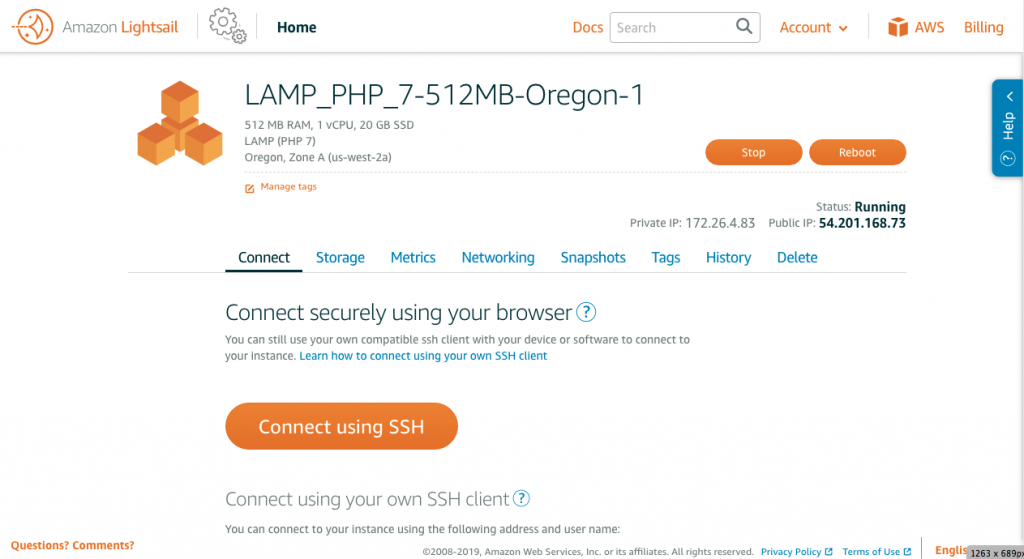
Now we need to connect to SSH terminal to perform some cool command line work. You can either use AWS website’s SSH portal (the Connect using SSH button on the previous picture) or use your own Command Prompt or Terminal.

If you connect using the later method, you need to download the SSH Key. To download it, click Account on the top bar, and click Account on the dropdown. Then, click SSH key and download it.

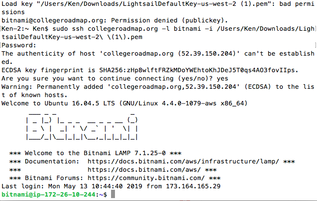
Use the following command to connect through SSH

ssh opportunityjunction.org(CAN USE IP AS WELL) -l bitnami -i PATH TO KEY FILE

After logging in the instance, you will see this screen on your Terminal.

Now you can perform Linux commands to the instance.

For a new created instance, I usually perform a routine update before doing anything.

sudo apt update && sudo apt upgrade

Setting server configuration for WordPress

When done, download wordpress and extract the package.

wget -c http://wordpress.org/latest.tar.gz
tar -xzvf latest.tar.gz

Now, you will get a wordpress file on your folder, if you perform the command.

ls

Next, you need to move the wordpress folder to /apps/ , where Bitnami instance usually stores website folder. You may rename it if you want.

sudo mv wordpress /apps/wordpress_opp

You need to set up the correct profile permission for it to work

chown daemon:daemon -R ./wordpress_opp
chmod 755 -R ./wordpress_opp

As you see, we set the ownership of the wordpress file to daemon. That’s what the

Before we started the installation process, we also need to create a mysql database for WordPress.

You can find the password to login using the following commands.

cat ~/bitnami_credentials

Login MySQL by typing the following commands:

mysql -u root -p

Then, a prompt to enter password shows up, and enter the password you find in the previous step. In the MySQL console, create a database using the following SQL command.

CREATE DATABASE wordpress_opp;

Remember the database name you use, because we need it for the installation of wordpress, as well as the MySQL password. You can exit the MySQL concole using:

exit

Now, we are one step away from actually installing WordPress. We need to configure Apache2, the server software and make it point to our WordPress folder.

cd /opt/bitnami/apache2/conf/bitnami

This is where the configureation file locates. Then open the file using Vim editor.

sudo vim bitnami.conf

Press i to start editing. Find a block that is embraced by <VirtualHost _default_:80> and </VirtualHost>. For example, something like that:

<VirtualHost _default_:80>
   ServerName collegeroadmap.org
   DocumentRoot "/opt/bitnami/apps/wordpress_opp/"
  <Directory "/opt/bitnami/apps/wordpress_opp/">
    Options Indexes FollowSymLinks
    AllowOverride All
    <IfVersion < 2.3 >
      Order allow,deny
      Allow from all
    </IfVersion>
    <IfVersion >= 2.3 >
      Require all granted
    </IfVersion>
  </Directory>
  # Error Documents
  ErrorDocument 503 /503.html

  # Bitnami applications installed with a prefix URL (default)
  #Include "/opt/bitnami/apache2/conf/bitnami/bitnami-apps-prefix.conf"
</VirtualHost>

Change the path next to DocumentRoot and Directory to the path of the target WordPress folder. And comment out the “Include …” line near the bottom.

When you need to create a second/third/… site, you just need to copy and paste a new <VirtualHost> block and change the path to the right folder.

Type :w to save the file, and type :q to quit the Vim editor. Just restart the server before you are going to isntall.

sudo /opt/bitnami/ctlscript.sh restart

Installing WordPress

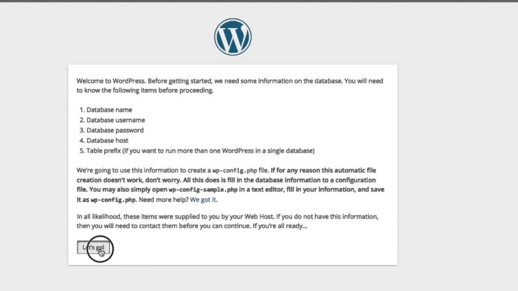
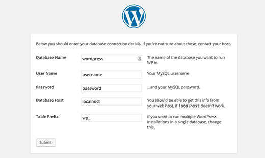
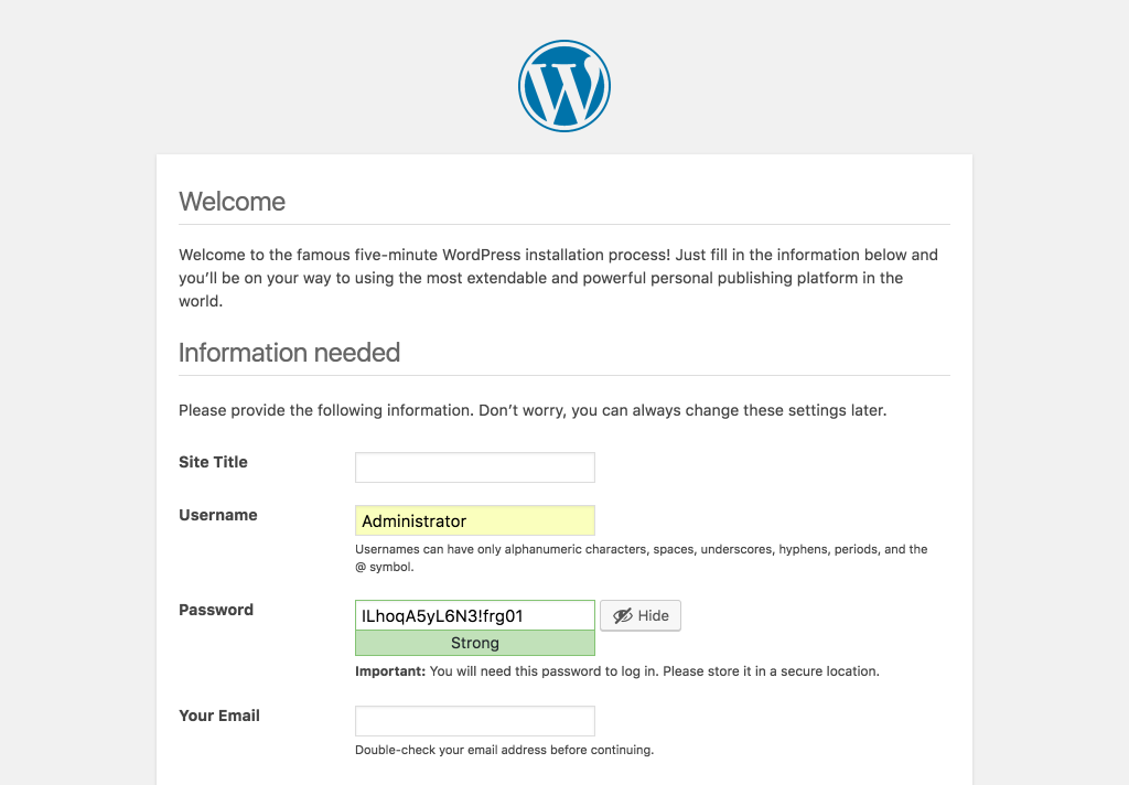
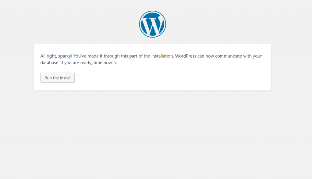
Visit the ip address or the URL (if you have pointed to the ip) of the server on the browser. If everything goes right, you will see the installation page. You just need to follow the instruction. During the process, you will need the MySQL database password and the name of the database you created.

On the above page, MySQL username is root, Database Host is localhost.

Wow, you made it! A new WordPress site has been installed. When you want to install a different site, just repeat the steps with a different folder name and database name.

Create SSL Certification using Let’s Encrypt

First, you need to stop apache2.

sudo /opt/bitnami/ctlscript.sh stop

Then, run this command to create the certificate to the default folder (or the one you chose).

sudo lego --tls --email="EMAIL-ADDRESS" --domains="DOMAIN" --domains="www.DOMAIN" --path="/etc/lego" run

At the same time, make sure to add these two lines to the apache2 config file that tells it where’s the certificate files.

SSLCertificateFile /etc/lego/certificates/xxxx.com.crt
SSLCertificateKeyFile /etc/lego/certificates/xxxx.com.key

Last, it’s to set up a routine to periodically renew the certificate. You can create a bash file (.sh) and set up a cron job for it.

#!/bin/bash
PATH=/usr/local/sbin:/usr/local/bin:/usr/sbin:/usr/bin:/sbin:/bin:/etc/lego/

sudo /opt/bitnami/ctlscript.sh stop apache
sudo /usr/local/bin/lego --tls --email='xxx' --domains='xxx.com'  --domains="www.xxxx.com" --path="/etc/lego" renew

echo "lego done"
sudo certbot --apache certonly -n -d mail.xxx.com
sudo certbot --apache certonly -n -d xxx.com

sudo cp /etc/lego/certificates/xxx.com.crt /home/bitnami/somewhere/server.crt
sudo cp /etc/lego/certificates/xxx.com.key /home/bitnami/somewhere/server.key

#sudo reboot
sudo /opt/bitnami/ctlscript.sh start apache

In the process there’re 3 and optionally 4 steps:

  • Stop the Apache process
  • Execute the renewal process
  • (optional) move the certicate to wherever needed
  • Start the Apache process

Setup SSL 443 Port in Apache Config

You need to add the following block to the apache config file.


<VirtualHost *:443>
  ServerName xxx.com
  ServerAlias www.xxx.com
  DocumentRoot "/opt/bitnami/abc/xxx"
  SSLEngine on           
  <Directory "/opt/bitnami/abc/xxx">
    Options Indexes FollowSymLinks
    AllowOverride All
    <IfVersion < 2.3 >
Order allow,deny
Allow from all
    </IfVersion>
    <IfVersion >= 2.3 >
Require all granted
    </IfVersion>
  </Directory>

Include "/opt/bitnami/apache2/conf/bitnami/bitnami-apps-prefix.conf"
  Include /etc/letsencrypt/options-ssl-apache.conf
SSLCertificateFile /etc/letsencrypt/live/xxx.com/fullchain.pem
SSLCertificateKeyFile /etc/letsencrypt/live/xxx.com/privkey.pem
</VirtualHost>

This block will tell the apache proxy where to look for the certificate file and what server name/alias to server. If you have set up a rewrite rule to route all HTTP to HTTPS. You can detele the :80 virtual host block mentioned above as well.

OLS Regression Model


OLS Regression Model


We will talk about Ordinary Least Square model in Python. In this article, we will just go over how to use OLS in Python without explaining the interpretation of the result.

Here, we will use sklearn and statsmodels packages to perform OLS modeling and compare the differences

In [105]:
from sklearn import linear_model as lm
import statsmodels.api as sm
from data_source_lib import *
from matplotlib import pyplot as pl

Use our data source class to get AAPL and SPY daily stock price

In [121]:
data_source = get_stock_data(tic_list=["AAPL","SPY"],freq = "daily")
data = data_source.get_ondemand_data()

# We can screen each stock by ticker names
AAPL = data[data.Ticker=="AAPL"]
SPY = data[data.Ticker=="SPY"]
Finished SPY
100%|████████████████████████████████████████████████████████████████████████████████████| 2/2 [00:00<00:00,  2.11it/s]

First, we will use sklearn package

In [109]:
# define the instance 
reg = lm.LinearRegression()
In [122]:
# Before applying the data, we should 
# turn it into numpy array

AAPL = np.array(AAPL[["close"]]) # we have imported numpy in our data source libary
SPY = np.array(SPY[["close"]])

# The reason I use SPY[["close"]] is to get 2D array
In [123]:
reg.fit(X=AAPL,y=SPY)
Out[123]:
LinearRegression(copy_X=True, fit_intercept=True, n_jobs=1, normalize=False)
In [124]:
reg.coef_
Out[124]:
array([[0.39143143]])
In [125]:
reg.intercept_
Out[125]:
array([199.09234191])

However, the sklearn package didn’t offer full statistic information in the OLS model. So we should use statsmodel instead for more information

Second, statsmodel Package

In [133]:
# This is to add a constant into the independent side of the model

AAPL2 = sm.add_constant(AAPL)
In [134]:
model = sm.OLS(SPY,AAPL2)
In [135]:
model = model.fit()
In [136]:
model.summary()
Out[136]:
OLS Regression Results
Dep. Variable: y R-squared: 0.639
Model: OLS Adj. R-squared: 0.636
Method: Least Squares F-statistic: 221.5
Date: Sun, 28 Oct 2018 Prob (F-statistic): 1.89e-29
Time: 23:33:17 Log-Likelihood: -383.96
No. Observations: 127 AIC: 771.9
Df Residuals: 125 BIC: 777.6
Df Model: 1
Covariance Type: nonrobust
coef std err t P>|t| [0.025 0.975]
const 199.0923 5.344 37.257 0.000 188.516 209.668
x1 0.3914 0.026 14.882 0.000 0.339 0.443
Omnibus: 35.484 Durbin-Watson: 0.103
Prob(Omnibus): 0.000 Jarque-Bera (JB): 59.620
Skew: -1.304 Prob(JB): 1.13e-13
Kurtosis: 5.114 Cond. No. 2.44e+03

Graphing/Plotting


There are a lot to say for graphing, or plotting. The package we used in Python is matplotlib, versus ggplot in R programming. In order to illustrate plotting, I also import numpy here to create some sample dataset.

In [4]:
from matplotlib import pylab as plt
import numpy as np

You can simply create plots like this:

In [28]:
x =np.linspace(-np.pi, np.pi, 255,endpoint=True)
# numpy's linespace function is pretty good at creating a x axis

y = np.sin(x)
plt.plot(x,y)
plt.show()
In [32]:
# Of course you can overlap plots

x =np.linspace(-np.pi, np.pi, 255,endpoint=True)
y = np.sin(x)
z = 2*x
plt.plot(x,y)
plt.plot(x,z)
plt.show()

Just need to make sure two plots run at the same time and they will be overlapped. At least one axis is the same among plots otherwise it will return an error.

If you want to customize the output, you need to do more.

Creating Subplot

You can have more than one plot in one canvas. The way to control it is to use subplot() method

The syntax for subplot is plt.subplot(No.row No.Col No.)

The top left plot of a 2×2 plot is plt.subplot(221)
The plot on its right is plt.subplot(222)

In [40]:
my_plot = plt.subplot(221) 
my_plot.plot(x,y)
# usually we store it into a variale for further formatting

my_plot2=plt.subplot(222) 
my_plot2.plot(x,z)

plt.show()

Setting The Plot Space

In [42]:
# Set the canvas
# The value in figsize is how many increments
plt.figure(figsize=(8,5), dpi=80)

my_plot = plt.subplot(111)
my_plot.plot(x,z)

# You can also set how the plot is being framed

my_plot.spines['right'].set_color('none')
my_plot.spines['top'].set_color('none')
my_plot.xaxis.set_ticks_position('bottom')
my_plot.yaxis.set_ticks_position('left')

# This property sets how the graph looks like
my_plot.spines['left'].set_position(('axes',0))
my_plot.spines['bottom'].set_position(("axes",0))

##### What if we change "axes" to" data"? 

plt.show()

And More

In [40]:
# Set the canvas
# The value in figsize is how many increments
plt.figure(figsize=(8,5), dpi=80)

my_plot = plt.subplot(111)

# You can also set color, line width, style and label
my_plot.plot(x,y,color="red", linewidth=1.5, linestyle="-", label="cosine")

# You can also set how the plot is being framed

my_plot.spines['right'].set_color('none')
my_plot.spines['top'].set_color('none')
my_plot.xaxis.set_ticks_position('bottom')
my_plot.yaxis.set_ticks_position('left')

# This property sets how the graph looks like
my_plot.spines['left'].set_position(('data',0))
my_plot.spines['bottom'].set_position(("data",0))


# I can also manipulate the axises 
plt.xlim(x.min()*1.1, x.max()*1.1) # set limits of current axis
plt.xticks([-np.pi, -np.pi/2, 0, np.pi/2, np.pi],
           [r'$-\pi

#39;, r‘$-\pi/2


#39;, r‘$0


#39;, r‘$+\pi/2


#39;, r‘$+\pi


#39;])
plt.ylim(y.min()*1.1,y.max()*1.1)
plt.yticks(range(10,10,1)
)
# annotate a specific point
plt.annotate(r‘$\sin(\frac{\pi}{2})=1


#39;,
xy=(np.pi/2,1), xycoords=‘data’,
xytext=(60, 40), textcoords=‘offset points’, fontsize=16,
arrowprops=dict(arrowstyle=“->”, connectionstyle=“arc3,rad=.2”))

plt.show()

Scatter Plot and More

In [44]:
import time
np.random.seed(int(time.time()))
#trial = [i for i in np.random.rand(100) ]
trial = np.array(np.random.rand(100))
y = trial *2
plt.scatter(trial,y)

# we can save the picture file
plt.savefig("test.png",dpi=72)

Histogram

Let’s get some finance data for this example

In [1]:
from data_source_lib import *

# import our magic lab
In [11]:
get_ins = get_stock_data(["AAPL"],freq= "daily",day_range=300)
my_data = get_ins.get_ondemand_data()["close"]
Finished AAPL
100%|████████████████████████████████████████████████████████████████████████████████████| 1/1 [00:00<00:00,  2.07it/s]
In [26]:
plt.figure(figsize=(8,5), dpi=80)
my_hist = plt.hist(my_data)
plt.xticks(range(50,300,10))
plt.show()

Technical Analysis

You may hear about Technical Analyst. That’s the basis of quantitative analysis of the stock market. There is a package in Python that makes the calculation of all the technical indicator much easier. I chose some of my favorite indicators and integrate into my code library.

Applying the talib is a little bit tricky, but take a look at this one line of code.

price.loc[price.Ticker==i,"ADXR"]= ta.ADXR(price.loc[price.Ticker==i].High.values, price.loc[price.Ticker==i].Low.values, price.loc[price.Ticker==i].Close.values, timeperiod=14)

The variable price is a DataFrame that return from our data getting object. Since we only want to analyze one stock’s time series feature, we want to filter the one ticker at one calculation, using price.Ticker == i. Then, the ADXR,  Average Directional Movement Index Rating indicator takes in High, Low and close. Basically, put them in the function of ta.ADXR()

For more information about the talib, check TA-Lib : Technical Analysis Library

Here’s the full picture of the function.


In [16]:
import talib as ta
import data_source_lib as da
In [15]:
get_data = da.get_stock_data(["AAPL"],freq = "daily")
price = get_data.get_ondemand_data()
Finished AAPL
100%|████████████████████████████████████████████████████████████████████████████████████| 1/1 [00:00<00:00,  1.56it/s]
In [40]:
 def get_technicals(price) :
    import pandas as pd
    import tqdm
    from IPython.display import clear_output
    if not isinstance(price, pd.DataFrame):
        raise "Please feed a DataFrame object"
    for i in tqdm.tqdm(range(len(set(price.Ticker)))):
       
       
        i = list(set(price.Ticker))
        #print price .loc[price.Ticker==i]

        #price.groupby('Ticker').get_group(list(set(price.Ticker))[i])
        #price.loc[price.Ticker==i,"ADX"]= ta.ADX(price.loc[price.Ticker==i].High.values, price.loc[price.Ticker==i].Low.values, price.loc[price.Ticker==i].Close.values, timeperiod=14)
        price.loc[price.Ticker==i,"ADXR"]= ta.ADXR(price.loc[price.Ticker==i].High.values, price.loc[price.Ticker==i].Low.values,\
                                                   price.loc[price.Ticker==i].Close.values, timeperiod=14)
        price.loc[price.Ticker==i,"APO"]= ta.APO(price.loc[price.Ticker==i].Close.values, fastperiod=12, slowperiod=26, matype=0)
        price.loc[price.Ticker==i,"AROONOSC"]= ta.AROONOSC(price.loc[price.Ticker==i].High.values,price.loc[price.Ticker==i].Close.values, timeperiod=14)
        price.loc[price.Ticker==i,"CCI"]= ta.CCI(price.loc[price.Ticker==i].High.values,price.loc[price.Ticker==i].Low.values,price.loc[price.Ticker==i].Close.values, timeperiod=14)
        price.loc[price.Ticker==i,"MFI"]= ta.MFI(price.loc[price.Ticker==i].High.values, price.loc[price.Ticker==i].Low.values, price.loc[price.Ti