How to Correctly Install CuDF for Python

Introduction of CuDF

CuDF is a powerful tool in the era of big data. It utilizes GPU computing framework Cuda to speed up data ETL and offers a Pandas-like interface. The tool is developed by the team, RapidAI

You can check out their Git repo here.

I love the tool. It gives me a way to make full use of my expensive graphic card, which most of the time only used for gaming. Most importantly, for a company like Owler, which has to handle 14 millions+ company profiles, even a basic data transformation task might take days. This tool is possible to help speed up the process by about 80+ times. GPU computing has been a norm for ML/AL. CuDF makes it also good for the upper stream of the flow, the ETL. And ETL is in high demand for almost every company with digital capacity in the world.

The Challenges

It’s nice to have this tool for our day-to-day data work. However, the convenience comes at a cost. That is, the installation of CuDF is quite confusing and hard to follow. It also has some limitations in OS and Python versions. Currently, it only works with Linux and Python 3.7+. And it only provides a condo-forge way to install; otherwise, you need to build from the source.

The errors range from solving environment fail, dependencies conflict, inability to find GPU, and such. I have been installing CuDF into a couple of servers, including personal desktop, AWS, and so on. Each time, I have to spend hours dealing with multiple kinds of errors and try them again and again. When it finally works, I don’t know which one is the critical step because there were so many variables. Most ugly, when you have dependency conflict error, you have to wait for a very long time after 4 solving environment attempts until it displays the conflicting package for you.

But the good news is, from the most recent installation, I can finally understand the cause for the complication and summarize an easy to follow guide for anyone who wants to enjoy this tool.

In short, the key is, use miniconda or create a new environment in anaconda to install.

Let me walk through the steps.

Installing the Nvidia Cuda framework (Ubuntu)

Installing Cuda is simple when you have the right machine. You can follow the guide here from Nvidia official webpage. If you encounter an installation error, please check if you are selecting the right architecture and meet the hardware/driver requirements.

However, if you have an older version of Cuda installed and wish to upgrade that. The Nvidia guide won’t help you anyway. The correct way is to uninstall the older version Cuda first before doing anything from the guide. The reason is that, at least in Ubuntu, the installation step will change your apt-get source library; once you do that, you will no longer be able to uninstall the older version, and it may cause conflict.

To uninstall Cuda, you can try the following steps. (for Ubuntu)

  • Remove nvidia-cuda-toolkit
sudo apt-get remove nvidia-cuda-toolkit

You may want to use this command instead to remove all the dependencies as well.

sudo apt-get remove --auto-remove nvidia-cuda-toolkit
  • Remove Cuda
sudo apt-get remove cuda

If you forgot to remove the older version cuda before installing the new version, you would need to remove all dependencies for cuda and start over the new version installation.

sudo apt-get remove --auto-remove cuda
  • Install cuda by following the Nvidia official guide. Link above.

Install CuDF

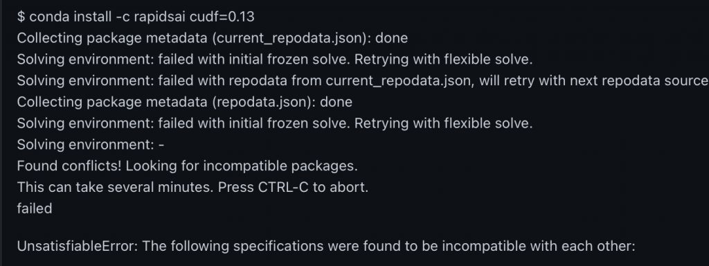
I highly recommend installing CuDF in miniconda. This will avoid most of the package dependency conflicts. If you have dependency conflicts, you will probably get the below error. Or you will be waiting forever during the last solving environment step.

Dependencies error

Miniconda is a much cleaner version of Anaconda. It has very few packages installed out of box. So it will avoid the CuDF installation running into conflict.

If you already have Anaconda installed and wish to keep it. You can try creating a new condo environment with no default package for CuDF.

conda create --no-default-packages -n myenv python=3.7

Pandas — Data Overviewing, Slicing and Selection


Untitled


Data Overview, Slicing and Selection

In [1]:
import pandas as pd
In [2]:
stock_data = pd.read_csv("pair_ETF_0302.csv")

When you read from raw data file, you get a Dataframe.

In [3]:
type(stock_data)
Out[3]:
pandas.core.frame.DataFrame

Data Overview

Get an overview of the data that you are working on. In this stage, you will focus on getting a board idea of data size, data type and information.

In [4]:
stock_data.head() #This is a function call, remember the ()
Out[4]:
pairs ave_return total_return volatility sharp_ratio
0 (‘NYT’, ‘BANC’) -1683.602874 -15.167593 139.660600 -0.108603
1 (‘EEA’, ‘ESS’) 7.915179 0.121772 123.131991 0.000989
2 (‘BXP’, ‘LFC’) 1194.149695 11.593686 88.070115 0.131642
3 (‘PCF’, ‘ANIK’) 2.441353 0.021605 13.484533 0.001602
4 (‘NDSN’, ‘POL’) -293.861701 -3.719768 36.593718 -0.101650
In [5]:
stock_data.tail()
Out[5]:
pairs ave_return total_return volatility sharp_ratio
58587 (‘INFO’, ‘MYF’) 1111.644206 8.964873 84.062452 0.106645
58588 (‘AL’, ‘CSL’) 917.521116 7.399364 63.715749 0.116131
58589 (‘PFL’, ‘DSW’) -876.763054 -7.070670 49.698238 -0.142272
58590 (‘HWBK’, ‘KRNY’) -106.253729 -0.856885 22.987587 -0.037276
58591 (‘AN’, ‘KAP’) 36.888918 0.297491 7.444777 0.039960

You can access columns the below methods

In [6]:
stock_data.pairs.head()
Out[6]:
0    ('NYT', 'BANC')
1     ('EEA', 'ESS')
2     ('BXP', 'LFC')
3    ('PCF', 'ANIK')
4    ('NDSN', 'POL')
Name: pairs, dtype: object
In [7]:
stock_data["pairs"].head()
Out[7]:
0    ('NYT', 'BANC')
1     ('EEA', 'ESS')
2     ('BXP', 'LFC')
3    ('PCF', 'ANIK')
4    ('NDSN', 'POL')
Name: pairs, dtype: object

You will get a data type of Series. You can view Series as a single unit of Dataframe.

In [8]:
type(stock_data["pairs"])
Out[8]:
pandas.core.series.Series

You can access specific cell like this.

In [9]:
stock_data["pairs"][0]
Out[9]:
"('NYT', 'BANC')"
In [10]:
type(stock_data["pairs"][0])
Out[10]:
str

Slicing and Selection

You can access a certain portion of data. Please remind that index starts from 0.

In [11]:
stock_data[:].head() #Showing all slices
Out[11]:
pairs ave_return total_return volatility sharp_ratio
0 (‘NYT’, ‘BANC’) -1683.602874 -15.167593 139.660600 -0.108603
1 (‘EEA’, ‘ESS’) 7.915179 0.121772 123.131991 0.000989
2 (‘BXP’, ‘LFC’) 1194.149695 11.593686 88.070115 0.131642
3 (‘PCF’, ‘ANIK’) 2.441353 0.021605 13.484533 0.001602
4 (‘NDSN’, ‘POL’) -293.861701 -3.719768 36.593718 -0.101650
In [12]:
stock_data[2:].head()  #start from the 3rd row
Out[12]:
pairs ave_return total_return volatility sharp_ratio
2 (‘BXP’, ‘LFC’) 1194.149695 11.593686 88.070115 0.131642
3 (‘PCF’, ‘ANIK’) 2.441353 0.021605 13.484533 0.001602
4 (‘NDSN’, ‘POL’) -293.861701 -3.719768 36.593718 -0.101650
5 (‘DAKT’, ‘LPG’) -578.896261 -5.122976 255.150999 -0.020078
6 (‘AGR’, ‘MXIM’) 2203.294225 21.600924 163.622809 0.132017
In [13]:
stock_data[:3] #get until the 4th row
Out[13]:
pairs ave_return total_return volatility sharp_ratio
0 (‘NYT’, ‘BANC’) -1683.602874 -15.167593 139.660600 -0.108603
1 (‘EEA’, ‘ESS’) 7.915179 0.121772 123.131991 0.000989
2 (‘BXP’, ‘LFC’) 1194.149695 11.593686 88.070115 0.131642
In [14]:
stock_data["pairs"].head()  # Usually I use column name to access column
Out[14]:
0    ('NYT', 'BANC')
1     ('EEA', 'ESS')
2     ('BXP', 'LFC')
3    ('PCF', 'ANIK')
4    ('NDSN', 'POL')
Name: pairs, dtype: object

More Slicing and Selection

This doesn’t work because it’s accessing the index, and the Dataframe doesn’t have the index named 0

In [15]:
stock_data[0] 
---------------------------------------------------------------------------
KeyError                                  Traceback (most recent call last)
<ipython-input-15-e3654389130b> in <module>()
----> 1 stock_data[0]

C:\ProgramData\Anaconda2\lib\site-packages\pandas\core\frame.py in __getitem__(self, key)
   2683             return self._getitem_multilevel(key)
   2684         else:
-> 2685             return self._getitem_column(key)
   2686 
   2687     def _getitem_column(self, key):

C:\ProgramData\Anaconda2\lib\site-packages\pandas\core\frame.py in _getitem_column(self, key)
   2690         # get column
   2691         if self.columns.is_unique:
-> 2692             return self._get_item_cache(key)
   2693 
   2694         # duplicate columns & possible reduce dimensionality

C:\ProgramData\Anaconda2\lib\site-packages\pandas\core\generic.py in _get_item_cache(self, item)
   2484         res = cache.get(item)
   2485         if res is None:
-> 2486             values = self._data.get(item)
   2487             res = self._box_item_values(item, values)
   2488             cache[item] = res

C:\ProgramData\Anaconda2\lib\site-packages\pandas\core\internals.py in get(self, item, fastpath)
   4113 
   4114             if not isna(item):
-> 4115                 loc = self.items.get_loc(item)
   4116             else:
   4117                 indexer = np.arange(len(self.items))[isna(self.items)]

C:\ProgramData\Anaconda2\lib\site-packages\pandas\core\indexes\base.py in get_loc(self, key, method, tolerance)
   3063                 return self._engine.get_loc(key)
   3064             except KeyError:
-> 3065                 return self._engine.get_loc(self._maybe_cast_indexer(key))
   3066 
   3067         indexer = self.get_indexer([key], method=method, tolerance=tolerance)

pandas\_libs\index.pyx in pandas._libs.index.IndexEngine.get_loc()

pandas\_libs\index.pyx in pandas._libs.index.IndexEngine.get_loc()

pandas\_libs\hashtable_class_helper.pxi in pandas._libs.hashtable.PyObjectHashTable.get_item()

pandas\_libs\hashtable_class_helper.pxi in pandas._libs.hashtable.PyObjectHashTable.get_item()

KeyError: 0
In [16]:
stock_data.iloc[0] #But you can access nth row using .iloc[n]
Out[16]:
pairs           ('NYT', 'BANC')
ave_return              -1683.6
total_return           -15.1676
volatility              139.661
sharp_ratio           -0.108603
Name: 0, dtype: object
In [17]:
type(stock_data.iloc[0]) #it returns a Series
Out[17]:
pandas.core.series.Series
In [18]:
stock_data.iloc[0:2] #You can also feed a portion to .iloc and it will return Dataframe
Out[18]:
pairs ave_return total_return volatility sharp_ratio
0 (‘NYT’, ‘BANC’) -1683.602874 -15.167593 139.660600 -0.108603
1 (‘EEA’, ‘ESS’) 7.915179 0.121772 123.131991 0.000989
In [19]:
stock_data.loc[[1,2]] #.loc can also be feeded a list of index
Out[19]:
pairs ave_return total_return volatility sharp_ratio
1 (‘EEA’, ‘ESS’) 7.915179 0.121772 123.131991 0.000989
2 (‘BXP’, ‘LFC’) 1194.149695 11.593686 88.070115 0.131642

Using .loc[], you can conduct more complex selection

In [20]:
stock_data.loc[:,"pairs"].head() # .loc can also be used to access columns 
Out[20]:
0    ('NYT', 'BANC')
1     ('EEA', 'ESS')
2     ('BXP', 'LFC')
3    ('PCF', 'ANIK')
4    ('NDSN', 'POL')
Name: pairs, dtype: object

Remember to feed a list when you want to select multiple columns or rows

In [21]:
stock_data.loc[:,["pairs","total_return"]].head()
Out[21]:
pairs total_return
0 (‘NYT’, ‘BANC’) -15.167593
1 (‘EEA’, ‘ESS’) 0.121772
2 (‘BXP’, ‘LFC’) 11.593686
3 (‘PCF’, ‘ANIK’) 0.021605
4 (‘NDSN’, ‘POL’) -3.719768
In [22]:
stock_data.loc[stock_data["ave_return"]>0].head()
Out[22]:
pairs ave_return total_return volatility sharp_ratio
1 (‘EEA’, ‘ESS’) 7.915179 0.121772 123.131991 0.000989
2 (‘BXP’, ‘LFC’) 1194.149695 11.593686 88.070115 0.131642
3 (‘PCF’, ‘ANIK’) 2.441353 0.021605 13.484533 0.001602
6 (‘AGR’, ‘MXIM’) 2203.294225 21.600924 163.622809 0.132017
8 (‘PUK’, ‘UTX’) 184.141559 1.629571 28.527874 0.057122

.loc is for index access, which means you should feed index or index generator into .iloc[]

In [23]:
stock_data.loc[[True,True,False]] #Boolean can be feeded into .loc, empty means false
Out[23]:
pairs ave_return total_return volatility sharp_ratio
0 (‘NYT’, ‘BANC’) -1683.602874 -15.167593 139.660600 -0.108603
1 (‘EEA’, ‘ESS’) 7.915179 0.121772 123.131991 0.000989

To use more complex selection, you can use lambda functions

In [24]:
stock_data.loc[lambda stock_data:stock_data["total_return"]>200000]
Out[24]:
pairs ave_return total_return volatility sharp_ratio
4684 (‘ITG’, ‘OIS’) inf inf NaN NaN
12016 (‘LEA’, ‘CTX’) 1.873543e+08 1.510922e+06 1.684723e+07 0.089684
24034 (‘ENVA’, ‘CTX’) 1.718711e+08 1.386057e+06 1.537679e+07 0.090140
34122 (‘TVPT’, ‘FULT’) inf inf NaN NaN
42235 (‘FOE’, ‘AOD’) inf inf NaN NaN
42749 (‘ALTR’, ‘EPD’) inf inf NaN NaN
46295 (‘FORM’, ‘AMSF’) inf inf NaN NaN
46678 (‘GS’, ‘ONB’) inf inf NaN NaN
54771 (‘NOV’, ‘CTX’) 1.789989e+08 1.443540e+06 1.601276e+07 0.090149

One Last Thing

As a good practice, you should always use .loc to set value. Because if you use direct access, like stock_data[“pairs”], Python will return a copy of the Dataframe, which is not changeable.

In [25]:
stock_data.loc[0,"ave_return"] = 0
In [26]:
stock_data.head()
Out[26]:
pairs ave_return total_return volatility sharp_ratio
0 (‘NYT’, ‘BANC’) 0.000000 -15.167593 139.660600 -0.108603
1 (‘EEA’, ‘ESS’) 7.915179 0.121772 123.131991 0.000989
2 (‘BXP’, ‘LFC’) 1194.149695 11.593686 88.070115 0.131642
3 (‘PCF’, ‘ANIK’) 2.441353 0.021605 13.484533 0.001602
4 (‘NDSN’, ‘POL’) -293.861701 -3.719768 36.593718 -0.101650

Series & Numpy Array

Pandas’s Series is internally Numpy Array. In the following demonstration, you will see if you take .values of the Series, you get an array.

In [30]:
stock_data.head()["pairs"].values
Out[30]:
array(["('NYT', 'BANC')", "('EEA', 'ESS')", "('BXP', 'LFC')",
       "('PCF', 'ANIK')", "('NDSN', 'POL')"], dtype=object)

Pandas — Reading Raw Data

Pandas is a powerful data organization and analysis toolbox in Python. It has functions and methods that can help you clean, organize and present data in much nicer way than any other data structures.

I will not be able to cover all Pandas functions/methods, but I would rather try to discover the logic and methodology underneath this package. So, you don’t need to remember everything but still be able to get things done efficiently.

First of all, I will talk about reading raw data from various sources using Pandas.

As you can see below, using pd.read_xxx, you can read various data file into Pandas.

Let’s take a close look at read_csv, which is the most common raw data file type.

One trick to get a first look at a method/function that you are using is to press TAB button, and it will show you all the available options.


Usually, you can just feed the file path to read the file.

But sometimes, you got broken data frame, and those reading options can help you get a better result.